
Microsoft Excel is an excellent number crunching software. If we needed tabulated data and statistics, it is one of the popular choices since it is a part of the MS Office package. In this tutorial I will introduce you to it’s built in capability to handle aggregated or summarized information using the formula toolbar.
When we say aggregated data, we mean grouped or calculated data coming from a set of data. The usual examples of aggregated data are average, median and mode while the more complicated are standard deviation and Poisson distribution.
To demonstrate how to use these formulas, I have created a dummy spread sheet with 10 items:

Note: those are arbitrary numbers for demonstration purposes only, you can use the steps that I will discuss on any set of numeric numbers you have on your sheet.
Let’s begin with calculating the average of these 10 numbers.
Step 1: Click on any part of the sheet where you want the average to appear
Step 2: Type the equal sign “=” then the word “average” followed by an opening parentheses “(“. You should see the “AVERAGE (number1, number 2…” tool tip appear if you have followed the steps correctly:

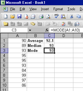
NOTE: The formula toolbar is the toolbar labeled with “fx” as shown above.
Step 3: Choose all the cells to be the range of data to be summarized. In this case I have cells A1 to cell A10. Close the parentheses to complete the parameter syntax:

Step 4: Hit ENTER key to see the output:

The formula toolbar will show you the formula used for that cell if you have your cursor pointed to that cell. You can see above that the average output of the 10 cells is 92.1. If you edit any of the 10 cells, the average value will automatically adjust.
Now for other formulas, follow the same step as above except the word “average”. So for median, it will be “=median(A1:A10)” while for mode it is “=mode(A1:A10)”:
Using the methods shown below, you will be able to easily create statistical reports and analysis using Excel. Excel can handle simple statistics that measure a central tendency like average, median and mode and it can also be used for more complex calculations using the same method done above.
Post a Comment